SageMath で楕円曲線を描いて、その上で楕円曲線上の加算の様子をグラフ (画像) にする方法について説明します。 加算や2倍算がどのように行われているかを説明するときに便利です。

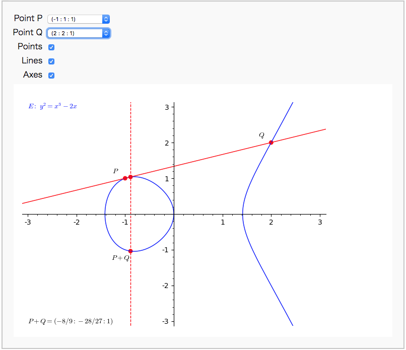
楕円曲線の式を点集合を直接プログラムに直書きして、「evaluate」ボタンを押すと、以下のようなセレクターとグラフ画像が出力されます。

点 $P$ と $Q$ の楕円曲線 $E$ 上の加算は、直線 $PQ$ と曲線 $E$ の交点をもとめて、その座標をx軸で折り返した点が $P + Q$ です。

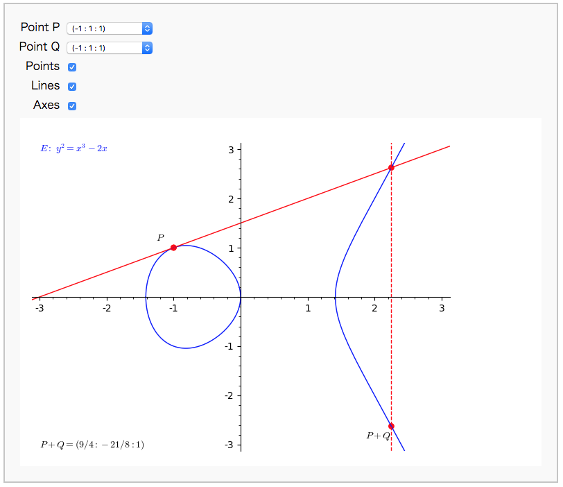
点 $P$ の楕円曲線上での2倍算は、曲線 $E$ の点 $P$ における接線と曲線 $E$ の交点をもとめて、その座標をx軸で折り返した点が $P + P = 2P$ です。 2倍算のグラフも以下のように正しく描画できています。

グラフの作り方は、まずSageMathを起動して、notebookを起動します。

$ sage
sage: notebook()

次に、notebook上でワークシート (Worksheet) を作成し、次のプログラムを入力＆実行します。

def point_txt(P, name, rgbcolor):
    if (P.xy()[1]) < 0:
        r = text(name, [float(P.xy()[0])-0.2, float(P.xy()[1])-0.2],
            rgbcolor=rgbcolor)
    elif P.xy()[1] == 0:
        r = text(name, [float(P.xy()[0])-0.2, float(P.xy()[1])+0.2],
            rgbcolor=rgbcolor)
    else:
        r = text(name, [float(P.xy()[0])-0.2, float(P.xy()[1])+0.2],
            rgbcolor=rgbcolor)
    return r

# 実数体上の楕円曲線 y^2 = x^3 - 2x
E = EllipticCurve([-2, 0])
list_of_points = [E(0, 0), E(-1,-1), E(-1 ,1), E(2, 2), E(2, -2), E(9/4, -21/8),
                  E(9/4, 21/8), E(-8/9, 28/27), E(-8/9, -28/27)]
html("Graphical addition of two points $P$ and $Q$ on the curve $ E: %s $ " % \
     latex(E))

@interact
def _(P=selector(list_of_points, default=list_of_points[2], label='Point P'),
      Q=selector(list_of_points, default=list_of_points[2], label='Point Q'),
      marked_points=checkbox(default=True, label='Points'),
      lines_on=checkbox(default=True, label='Lines'), Axes=True):
    if lines_on:
        Lines = 2
    else:
        Lines = 0
    curve = E.plot(rgbcolor=(0, 0, 1), xmin=-25, xmax=25, plot_points=300)
    R = P + Q
    Rneg = -R
    if R == E(0):
        l1 = line_from_curve_points(E, P, Q)
        p1 = plot(P, rgbcolor=(1, 0, 0), pointsize=40)
        p2 = plot(Q, rgbcolor=(1, 0, 0), pointsize=40)
        textp1 = point_txt(P, "$P$", rgbcolor=(0, 0, 0))
        textp2 = point_txt(Q, "$Q$", rgbcolor=(0, 0, 0))
        if Lines == 0:
            g = curve
        elif Lines == 1:
            g = curve + l1
        elif Lines == 2:
            g = curve + l1
        if marked_points:
            g = g + p1 + p2
        if P != Q:
            g = g + textp1 + textp2
        else:
            g = g + textp1
    else:
        l1 = line_from_curve_points(E, P, Q)
        l2 = line_from_curve_points(E, R, Rneg, style='--')
        p1 = plot(P, rgbcolor=(1, 0, 0), pointsize=40)
        p2 = plot(Q, rgbcolor=(1, 0, 0), pointsize=40)
        p3 = plot(R, rgbcolor=(1, 0, 0), pointsize=40)
        p4 = plot(Rneg, rgbcolor=(1, 0, 0), pointsize=40)
        textp1 = point_txt(P, "$P$ ", rgbcolor=(0, 0, 0))
        textp2 = point_txt(Q, "$Q$", rgbcolor=(0, 0, 0))
        textp3 = point_txt(R, "$P+Q$", rgbcolor=(0, 0, 0))
        if Lines == 0:
            g = curve
        elif Lines == 1:
            g = curve + l1
        elif Lines == 2:
            g = curve + l1 + l2
        if marked_points:
            g = g + p1 + p2 + p3 + p4
        if P != Q:
            g = g + textp1 + textp2 + textp3
        else:
            g = g + textp1 + textp3
    g = g + text("$P+Q=%s$" % R, [-3, -3], rgbcolor=(0, 0, 0),
                 horizontal_alignment="left")
    g = g + text("$E: \ %s$" % latex(E), [-3, 3],
                 horizontal_alignment="left")
    g.axes_range(xmin=-3, xmax=3, ymin=-3, ymax=3)
    show(g, axes=Axes)

def line_from_curve_points(E, P, Q, style='-', rgb=(1, 0, 0), length=25):
    """
    P,Q two points on an ellipticcurve.
    Output is a graphic representation of the straight line
        intersecting with P,Q.
    """
    # The function tangent to P=Q on E
    if P == Q:
        if P[2]== 0:
            return line([(1, -length), (1, length)],
                        linestyle=style, rgbcolor=rgb)
        else:
            # Compute slope of the curve E in P
            [a1, a2, a3, a4, a6] = E.a_invariants()
            numerator = (3*P[0]**2 + 2*a2*P[0] + a4 - a1*P[1])
            denominator = (2*P[1] + a1*P[0] + a3)
            if denominator == 0:
                return line([(P[0], -length), (P[0], length)],
                            linestyle=style, rgbcolor=rgb)
            else:
                l = numerator / denominator
                f(x) = l * (x - P[0]) + P[1]
                return plot(f(x), (-length, length),
                            linestyle=style, rgbcolor=rgb)
    # Trivial case of P != R where P = O or R = O then we get the
    # vertical line from the other point
    elif P[2] == 0:
        return line([(Q[0], -length), (Q[0], length)],
                    linestyle=style, rgbcolor=rgb)
    elif Q[2] == 0:
        return line([(P[0], -length), (P[0], length)],
                    linestyle=style, rgbcolor=rgb)
    # Non trivial case where P != R
    else:
        # Case where x_1 = x_2 return vertical line evaluated in Q
        if P[0] == Q[0]:
            return line([(P[0], -length), (P[0], length)],
                        linestyle=style, rgbcolor=rgb)

        # Case where x_1 != x_2 return line trough P,R evaluated in Q"
        l = (Q[1] - P[1]) / (Q[0] - P[0])
        f(x) = l * (x - P[0]) + P[1]
        return plot(f(x), (-length, length),
                    linestyle=style, rgbcolor=rgb)

入力して「evaluate」ボタンを押すと、セレクターとグラフ画像が出力されます。

実数体上の楕円曲線の式をいろいろ変えてみると面白いかもしれません。 自分で試してみましょう！

以上です。